Bing Maps: Penetration Mapping
Added in Q4 2023
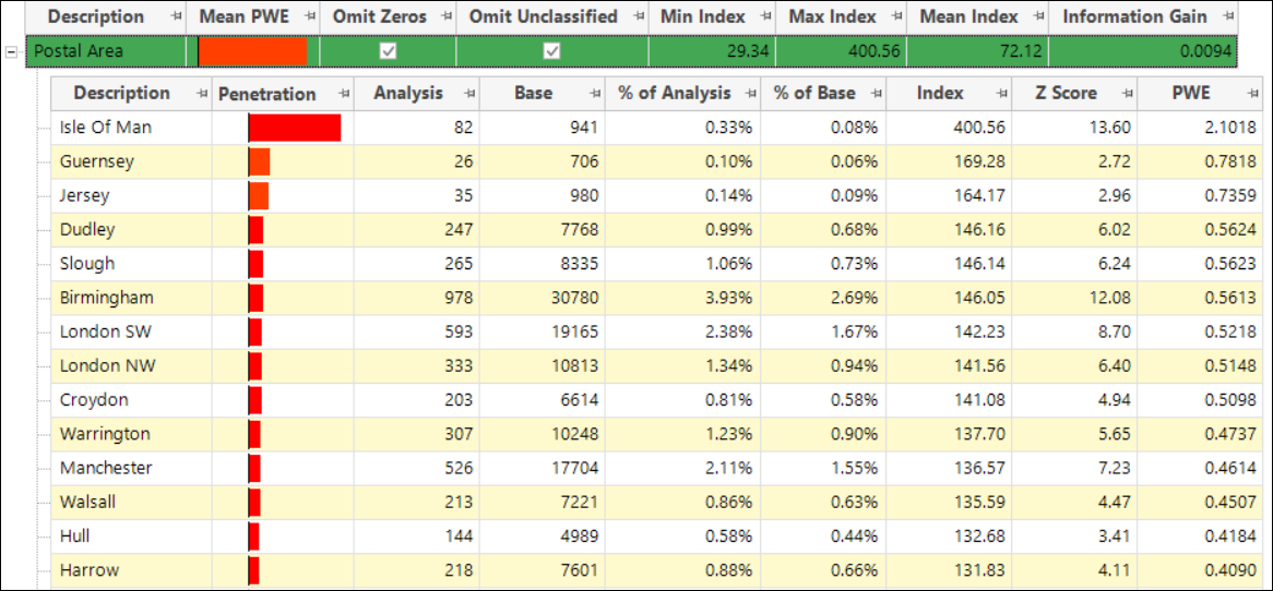
Penetration mapping compares particular groups of customers by location. This functionality builds upon the capabilities of the modelling Profile tool which allows you to make comparisons between two groups of people and examine a range of statistics. For example, the profile displayed below compares people who have made a booking to Sweden with the database as a whole, and the Postal Area variable has been added as a dimension of interest. You can see the over- and under-representation in each category very visually in the Penetration column, together with the supporting metrics.
Whilst this provides excellent insight, and allows you to identify categories of significance and interest, it is not possible to display the locations of the postal areas within the Profile tool itself and it is difficult to get a sense of how each area relates to the others.
Instead, within the Map tool, a new Selections option, accessed via the mapping toolbar, lets you specify an Analysis selection, optionally a Base selection, and one of the calculated insight measures which is then displayed for each geographical unit on the map.
Let’s take a look.
-
Open a new Map.
-
In the Layer 1 tab, add Postal Area as the geographic variable to use and build.
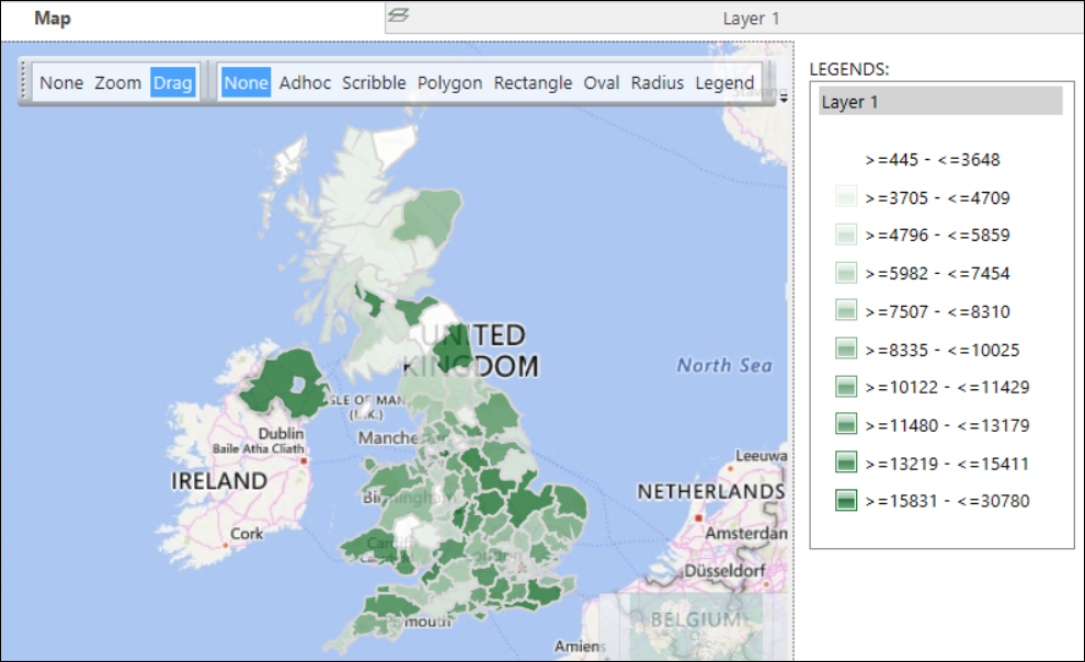
With no underlying selection, the resulting map displays the number of people on our database living in each UK postal area. The insight is limited. For example, the fact that London contains more people, and mid-Wales less, is linked to the fact that they are more and less populated anyway.
Penetration mapping offers greater insight:
-
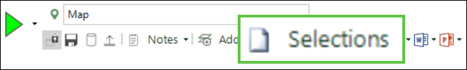
Click Selections on the map toolbar.
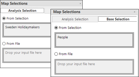
The Map Selections dialogue opens with two tabs.
-
Within the Analysis Selectiontab, drag and drop the selection of Sweden Holidaymakers into the From Selection drop-box.
-
Switch to the Base Selection tab where you can see that the default is People - i.e. all people on the database. Leave as the default.
At the bottom of the dialogue you can select the calculated insight metric from the Measure To Display drop-down:

-
Select Analysis Base Index and OK.
-
Rebuild the map.
You can see that the shading has updated and hovering over a postal area displays the corresponding index value. Here, the index values indicate that the areas around London, Birmingham and Manchester have a higher penetration and mid-Wales lower, suggesting that Sweden holidaymakers are generally located in more urban areas, although there are clearly some outliers, such as the Isle of Man, Glasgow and Hull.

Adding further measures
You can add other measures into the map to gain further insight. For example, you might want to compare the average cost of holidays for Sweden holidaymakers against the average cost of holidays for all customers and return the index value on this basis.
-
Switch to the map’s Layer 1 tab.
-
Right drag and drop the booking Cost variable onto the Statistics panel and select Mean(Cost).
-
Make Mean(Cost) the primary statistic and rebuild the display.

You can very quickly and easily discern that the average holiday values for each group demonstrate a very different pattern with, for example, north Wales and the south of Scotland being more over-represented compared to the customer base as a whole.
The available index measures and ratios can be applied to any of the statistics you have listed within the Layer 1 Statistics panel.
Added in Q2 24
A thematic shading has been introduced specifically for index measures. This development offers greater power and insight, providing a more natural way of applying shading symmetrically around the fixed threshold value of 100, with the maximum deviation in each direction linked, and ranges either side of the threshold being of the same size.
Take the Analysis Base Index penetration map example above:
-
In the Layers panel, select Thematic to access the Edit layer thematic dialogue.
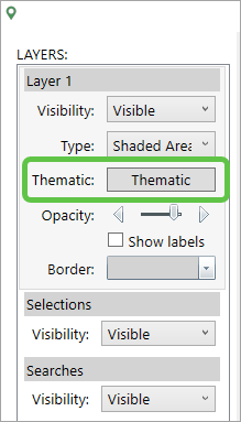
-
From the Type drop-down, select Index shading.
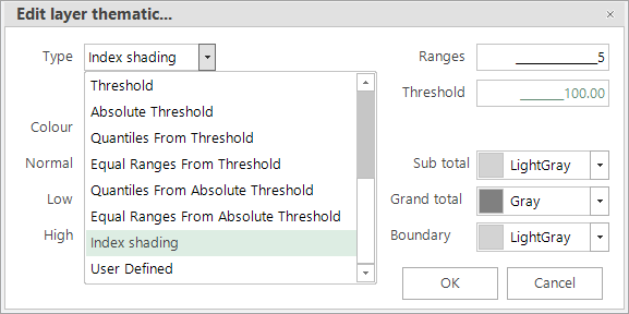
-
Select appropriate thematic colours - in this example, shades of blue for values below 100 and shades of red above.
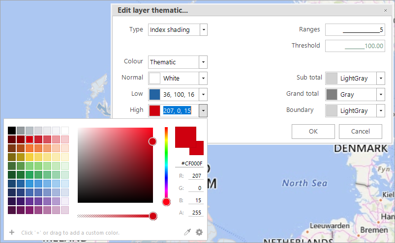
-
Set the number of ranges to 5 and click OK to update the map display.
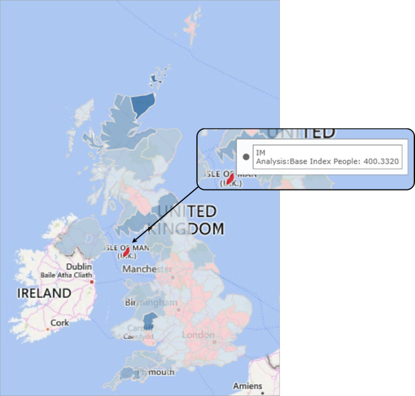
The insight? You can clearly see the under and over representation of Sweden Holidaymakers v All People by Postal Area. Whilst representation in most areas appears to be about average, the Isle of Man is strongly overrepresented and there are several areas - from Plymouth in the south west, to Llandrindod Wells in Wales and Kirkwall in Scotland which are quite significantly underrepresented.
Related topics:
Bing Maps: Penetration Mapping with Z-Scores
Bing Maps: Penetration Mapping - comparing records against an outside population