Cube: How do I use and interpret the different statistics?

The following example is based on a cube of Income vs Occupation for people living in Yorkshire and Humber.

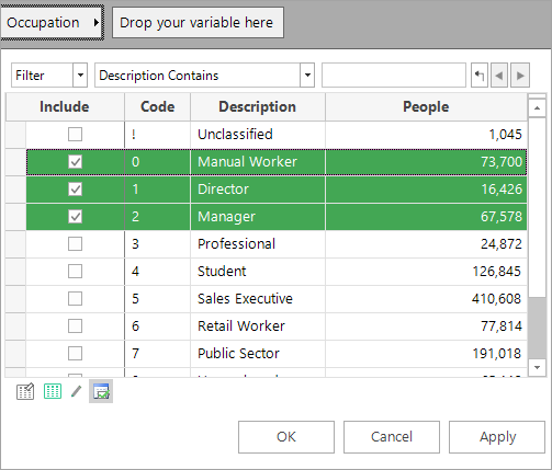
The occupation filter has been set to just show the 3 occupations.  The cube has been left on the default resolve level of People.

The different statistics highlight various characteristics of the data.  These are summarised below and explained in more detail in the following sections.  For more details on how the statistics are calculated or obtained in a cube.  See Cube: How do I include Statistics in a Cube?

Statistic	Description
Counts	Enables comparisons across all categories at an absolute level
% Column	Enables the relative patterns between columns to be discovered, adjusting for differences in column scale
% Row	Enables the relative patterns between rows to be discovered, adjusting for differences in row scale
% Total	Enable comparisons across all categories, as a percentage of the records in the underlying selection.
% Grand Total	Calculates the percentage of the value in this cell with reference to the grand total.
% Universe	Enable comparisons across all categories, as a percentage of all records at the resolve level.
Index	Shows size, direction, but not significance of unexpected results.  (Centred on 100, not symmetrical)
∑ Row	Enables progressive comparisons of the absolute counts, rather than column by column comparisons
∑ Column	Enables progressive comparisons of the absolute counts, rather than row by row comparisons
∑% Row	Enables progressive comparisons of the absolute counts, adjusting for differences in row scale
∑% Column	Enables progressive comparisons of the absolute counts, adjusting for differences in column scale
PWE	Shows size, direction, but not significance of unexpected results.  (Centred on 0, is symmetrical)
Chi Square	Shows size, significance , but not direction of unexpected results
Expected	Used in calculating subsequent statistics - shows counts expected if average distributions followed
ZdExp	Shows size, direction, and significance of unexpected results.  (Centred on 0, is symmetrical)
%d Exp	Shows size, direction, but not significance of unexpected results.  (Centred on 0, not symmetrical)

Counts

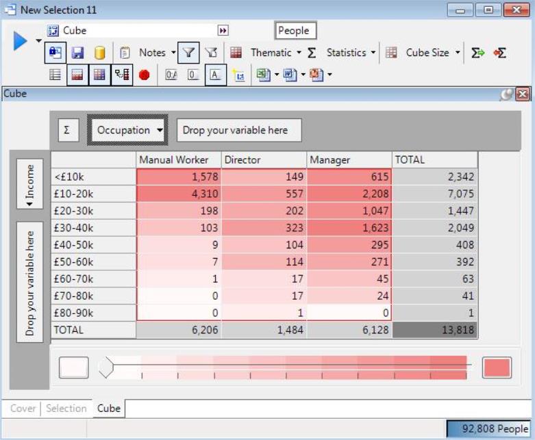
The Count displays the number of records in the underlying selection in each cell of the cube. The row total, column total and total cells sum the number of records across all the respective categories displayed in the cube.

The counts enable comparisons across the displayed categories at an absolute level. For example, we can learn that:

• There are roughly the same number of Managers (6,128) as Manual Workers (6,206) in the selected region.

• There are more Manual Workers on <£10k (1,578) than the total number of Directors (1,484).

• There are roughly the same number of Manual Workers on £20-30k (198) as there are Directors in this income band (202).

We are unable to determine relative patterns. For example, we cannot see:

• Which occupations have similar income distributions, since the counts are on totally different scales (e.g. 100s of Directors, but 1000s of Managers).

We are unable to see what is unusual about the different income-occupation combinations. For example:

• Is it more unusual to have 200 Manual workers on £20-30k or to have 200 Directors on this income band?

% Column

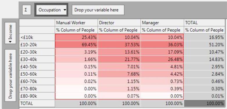
The % Column statistic overcomes the differences in scale between the columns (i.e. 100s of Directors in each income band, but 1000s of Managers - see Counts). The statistic is calculated by dividing the count for a cell by the total count for that column.

The % Column enables the relative patterns between columns to be discovered. For example:

• Managers and Directors have a similar income distribution, with a higher proportion of the higher incomes.

• The row totals column gives the average income distribution across the 3 occupations displayed.

By comparing the distributions of each occupation against the average, we can gain some insight. For example:

• Manual Workers have more than the average number of people in the £10-20k band (69% compared to 51%).

We can do some mental calculations to get a sense of which differences are most pronounced. However, some of the other statistics do this job for us, to show the size, and significance of these differences.

% Row

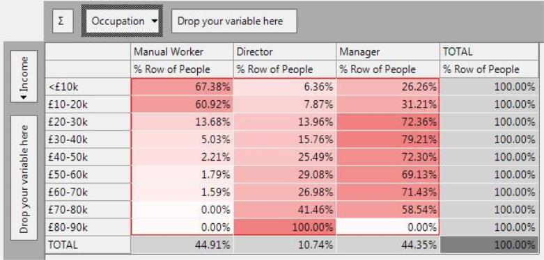
The % Row overcomes the differences in scale between the rows (i.e. 10s of people in the £70k+ bands, but 100s in the lower bands - see Counts). The statistic is calculated by dividing the count for a cell by the total count for that row.

The % Row enables the relative patterns between rows to be discovered. For example:

• Managers and Directors make up a similar proportion of the higher income bands (typically around 25-30% are Directors and 70% are Managers).

• Overall Manual Workers and Managers make up a similar percentage of the total workforce in this region (44.91% and 44.35%).

By comparing the distributions of each income band against the average, we can gain some insight. For example:

• Although Manual Workers and Managers make up a similar proportion of the total workforce, the lower income bands are dominated by Manual Workers and the higher income bands are dominated by Managers.

We can do some mental calculations to get a sense of which differences are most pronounced. However, some of the other statistics do this job for us, to show the size and significance of these differences.

% Total

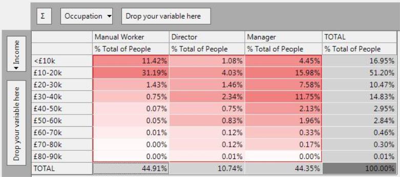
The % Total expresses the count in each cell as a percentage of the sub-total count in the cube. The sub-total figures are those within the red lined area of the cube. This total will only include records that satisfy the selection underlying the cube (in this case people living in Yorkshire and Humber).

% Grand Total

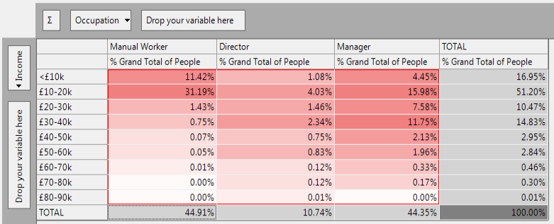
The % Grand Total expresses the count in each cell as a percentage of the total count in the cube. This total will only include records that satisfy the selection underlying the cube (in this case people living in Yorkshire and Humber).

% Universe

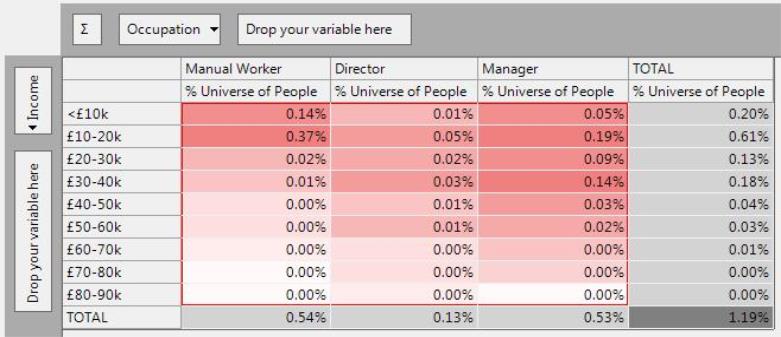
The % Universe expresses the count in each cell as a percentage of the total number of records at the resolve level and does not consider the selection underlying the cube.

Index

The Index is a ratio measure which gives an indication of the size and direction of any differences from the expected (but no indication of the significance).  It shows unusual values in the data, where there is some sort of relationship that is causing a difference from the average.  It is centred about 100, but is not symmetrical (see below).

The index is calculated by dividing the actual count by the expected count (x 100).  The same result is obtained by dividing the % Column  for a cell by the % Column for that row.

The interesting cells above are the dark red (high index) and also the very light ones (low index).  Using the index, we can see for example:

• The number of Directors with a £70-80k income is just under 4 times what you would expect if Directors had an average income distribution. Looking back at the counts and the expected, we see that we expected 4.4 but actually had 17. We will see from the ZdExp that this is not the most significant result.

• The number of Manual Workers with an income of £60-70k is 28 times less than you would expect. (Index of 3.53 = 100/3.53 = 28 times lower). Again, looking back at the counts, shows that this index has arisen from 1 person having this income when 28 were expected.

• The number of Manual Workers with an income of less than £10k is higher than would be expected – an index of 150.02. In other words the proportion of Manual Workers with this income is 50% higher than the average. (% Column is 25.43% instead of 16.95%)

The index is centred on100 (the %d Exp measure is very similar, but is centred on 0).  Being a ratio measure it is not symmetrical, in that an index of 300 (i.e. 200 above the norm of 100) is 3 times the expected, but an index of 20 (i.e. 80 below the norm of 100) is actually 5 times less than expected.  The under-indexing values are effectively squashed into the range 0 to 100, whereas the over-indexing values can extend indefinitely.  Care needs to be taken when interpreting these values.  The PWE value provides similar information but is symmetrical (about 0).

From the examples above, the high and low indices are often based on combinations with very low counts.  The ZdExp and Chi Square can be used to see if these differences are actually significant.

∑ Row - Cumulative Row Count

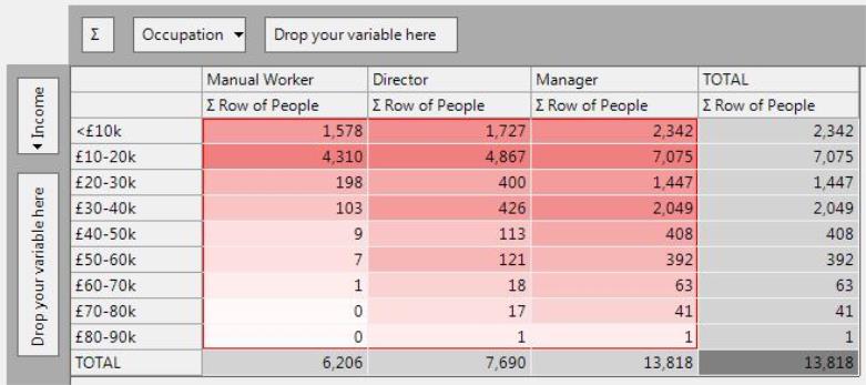
The cumulative row count aggregates the counts along the rows.

This enables progressive comparisons of the absolute counts, rather than column by column comparisons.  

See Cumulative Column Count for an example.

∑ Column - Cumulative Column Count

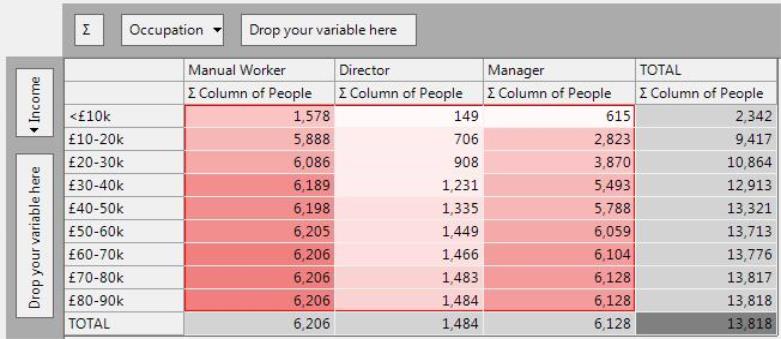
The cumulative column count aggregates the counts down the columns.

This enables progressive comparisons of the absolute counts, rather than row by row comparisons.  For example:

• There are only 2,823 Managers with an income of £20k or less, which is under half the number of Manual Workers in this income range (5,888).

∑% Row - Cumulative Row Percent

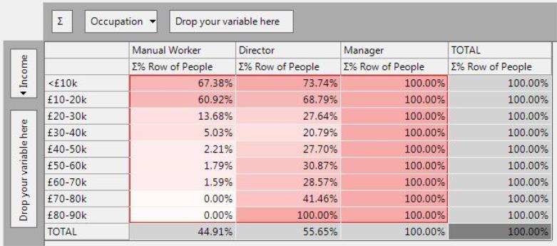
The cumulative row percent aggregates the counts along the rows and expresses each count as a percentage of the row total.

This removes the differences in scale between the rows (i.e. 10s of people in the £70k+ bands, but 100s in the lower bands).  and enables progressive comparisons of the relative distributions.  

See Cumulative Column Percent for an example.

∑% Column - Cumulative Column Percent

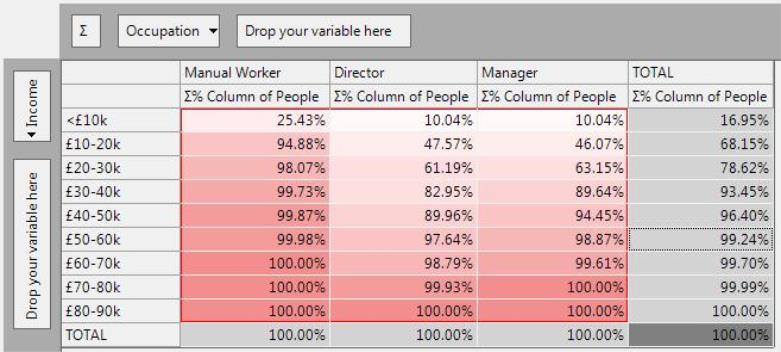
The cumulative column percent aggregates the counts down the columns and expresses each count as a percentage of the column total.

This removes the differences in scale between the columns (i.e. 100s of Directors in each income band, but 1000s of Managers) and enables progressive comparisons of the relative distributions.  

For example:

• The proportion of Managers with an income of £50k or less is higher than that for Directors (94.45% compared to 89.96%), indicating that the proportion of Managers with an income of £50k or above is less than that for Directors (5% compared to 10%).

PWE

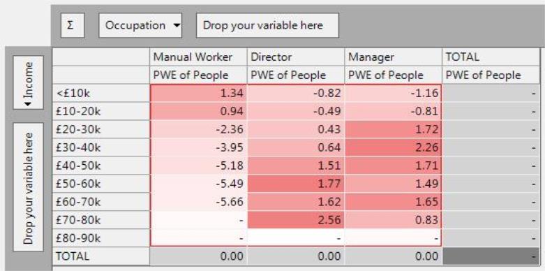
The PWE is the "Predictive Weight of Evidence", an additive measure which gives an indication of the size and direction of any differences from the expected (but no indication of the significance).  It shows unusual values in the data, where there is some sort of relationship that is causing a difference from the average.  It is centred about 0, and is symmetrical (see below).

The PWE calculation involves a log transformation to make the values symmetrical about 0, but at a fundamental level is similar to an index measure in that it compares the distribution within say a column to the average distribution.

The interesting cells above are again the dark red (high PWE) and also the very light ones (low PWE).  Using the PWE, we can gather all the same insight as we obtained from the index , but it is easier to compare the extent of the over and under representation:

• The PWE is positive for Directors with a £70-80k income (2.56) showing that this higher than would be expected if Directors had an average income distribution. Looking back at the counts and the expected, we see that this is based on very few people and again we will see from the ZdExp that this is not the most significant result.

• The PWE is negative for Manual Workers with an income of £60-70k (-5.66) showing again that they are unlikely to have such high incomes.

The symmetry of the PWE score means we can make a direct comparison of the absolute scores and since 5.66 is bigger than 2.56 it is clear that this is a larger under-representation (index showed 16 times lower than expected), than the above over-representation of Directors with a £70-80k (index showed only 4 times higher than expected).

Again the high and low values are often based on combinations with very low counts.  The ZdExp and Chi Square can be used to see if these differences are actually significant.

Chi Square

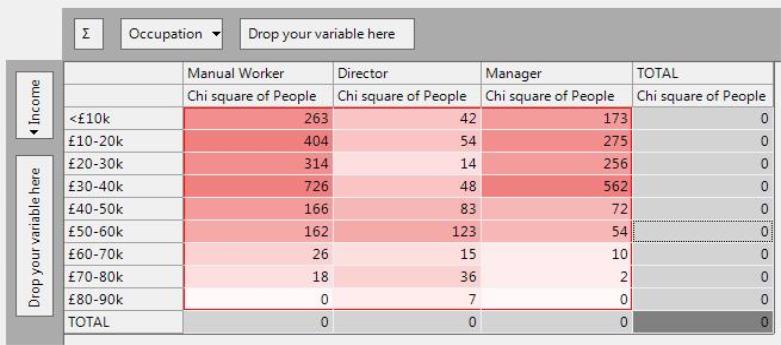
The Chi Square is a significance measure which gives an indication of both the size and significance of any differences from the expected, but it does not show the direction of these differences.  Values are always positive, and higher values indicate a difference based on a large number of records.

The Chi Square is calculated by taking the difference between the count and the expected, and squaring the result.

The Chi Square confirm the observations made based on the ZdExp:

• The most significant observation is that the number of Manual Workers in the £30-40k income band is very different from an expectation based on the average (high value of 726). However, the Chi Square is always positive, so we cannot deduce from this that it is an over-representation.

• Manual Workeres are over-represented in the less than £10k income band with a similar level of significance as the under-representation of Managers in the £10-20k band (Chi Square of 263 compared to 275).

Expected

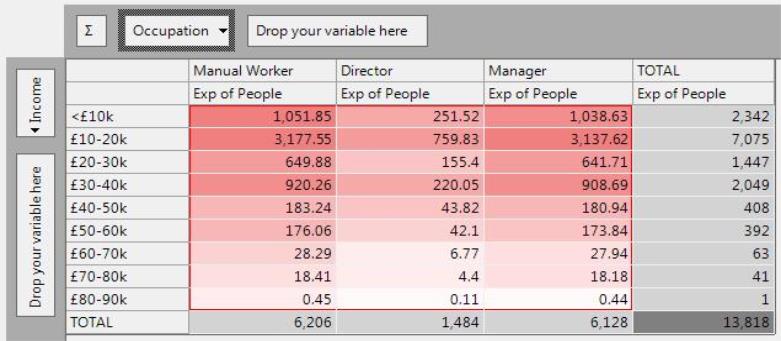
The Expected statistic tells you how many people you might expect in each income band of each occupation, if you were working from the assumption that each occupation followed an average income distribution.  

For example:

• Since the overall number of Manual Workers and Managers are similar, the expected number of each in the £10-20k band is similar (around 3,200). This figure has been calculated by applying the % row from the totals column (51.2%) to the column totals for each occupation.

• In other words, we expect 51.2% of each occupation to be in the £10-20k band. For Manual Workers, this is 51.2% x 6,206 = 3177.55.

The % Column and % Row statistics indicate that there are differences in the Income distributions of each occupation.  So far we have been able to see what these differences are (e.g. less Manual Workers in the higher income bands), but have not been able to quantify the size or significance of these differences.  The Expected values are a means to this end.  In themselves they are not very interesting but they are the basis of a number of useful statistics.

ZdExp

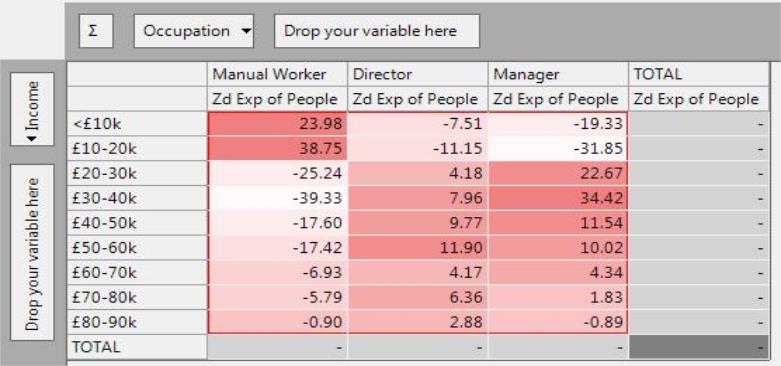
The ZdExp is the “z-score of deviation from expected value” and is a significance measure which gives an indication of both the size, direction and significance of any differences from the expected.  Positive values are due to higher counts than expected and negative values due to lower counts than expected.

The ZdExp again shows unusual values in the data, but the ZdExp value will be moderated if these differences are based on only a few records.  For example:

• The ZdExp confirms that Directors have a higher than average income (shown by positive values). However, the ZdExp for Directors with £80-90k income is "only" 2.88, (by no means the highest value in the cube), whereas this cell had the highest index value.

• The ZdExp value for Manual Workers with less than £10 income is again positive (reaffirming the higher than expected count as deduced from the index of 150). However, the much higher value (of 23.98) emphasising the higher volume of people in this category (count of 1,578).

• The most significant observation is that Managers are over-represented in the £30-40k income band.

Indices over 100 will always have a positive ZdExp, and both these facts indicate a relationship in the data (in this case that a certain occupation has more people in the income band than average).  However, the ZdExp also captures information about how many people this observation is based on.  Thus a very high index, that is only based on a few people, may have a lower ZdExp than a lower index (but still above 100) that is based on lots of people.

%d Exp

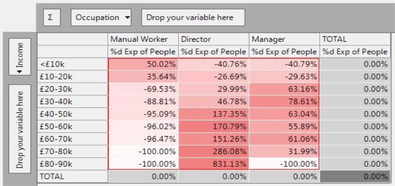
The %d Exp is the “percentage deviation from expected value”, a ratio measure which gives an indication of the size and direction of any differences from the expected (but no indication of the significance).  It shows unusual values in the data, where there is some sort of relationship that is causing a difference from the average.  It is centred about 0, but is not symmetrical (see below).

The %d Exp is calculated by dividing the difference between the actual count and the expected, by the expected count (x 100).  The same result is obtained by subtracting 100 from the index value.

The insight gained from the %d Exp is essentially the same as that from the Index measure, since the values are centred on 0 instead of 100, but are otherwise the same.  It perhaps is clearer from the %d Exp which cells are under-indexing, since they stand out as a result of the minus sign.  

Again the under-indexing values are effectively squashed into the range -100 to 0, whereas the over-indexing values can extend indefinitely.  Care needs to be taken when interpreting these values.  The PWE value provides similar information but is symmetrical (about 0).

Again the high and low values are often based on combinations with very low counts.  The ZdExp and Chi Square can be used to see if these differences are actually significant.