Cube: How do I include Statistics on a Cube?
By default a cube will show the record count, but you can specify different or additional information to display, including Calculated Measures.
To display different information:
-
Click the
 button. This
will show the above dialogue where, by
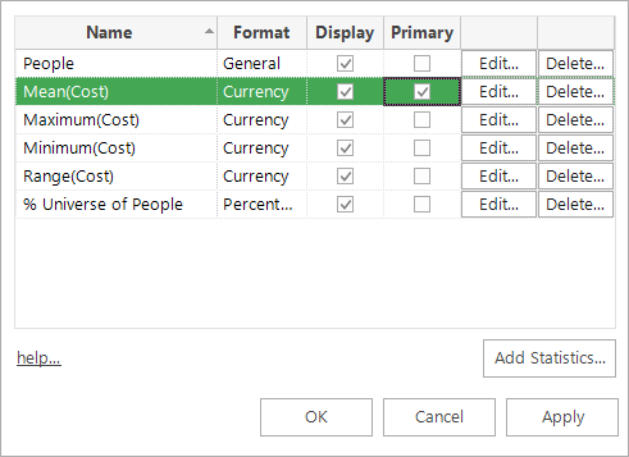
default, you will only see the "Count" figure.
button. This
will show the above dialogue where, by
default, you will only see the "Count" figure.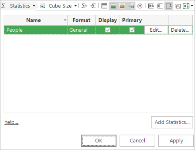
-
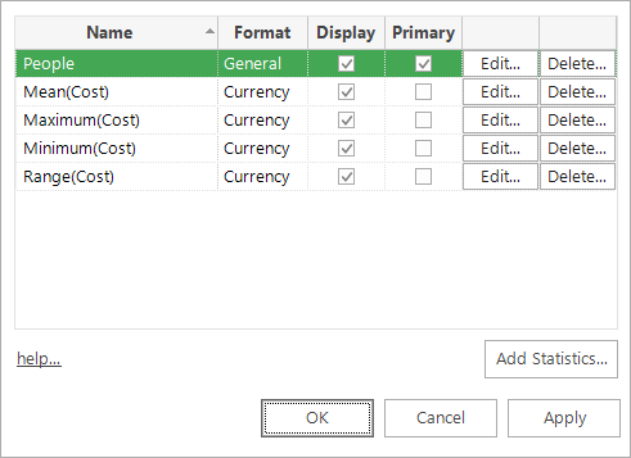
Select Add Statistics... to bring up the dialogue box that allows you to choose what other quantity you want to display.
.png)
-
Using the radio buttons, select whether you want to use the cube's resolve table for the count or whether you want to drag on some other item.
-
If you want to use another item, you can either drag on a different table, variable or expression. With variables and expressions you can also specify the function to use for aggregating the values.
-
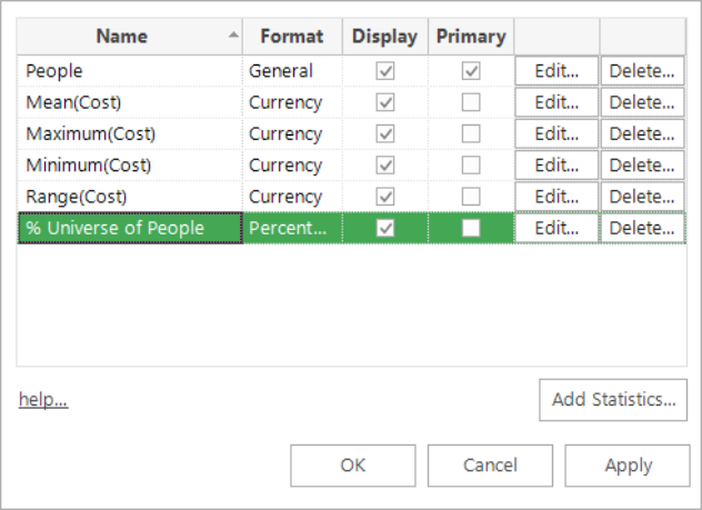
Then, regardless of the above choice, you can further specify whether you want to see just the value, or another statistic (such as the value as a percentage of the universe, etc). Press OK and this will be added to the list displayed.
-
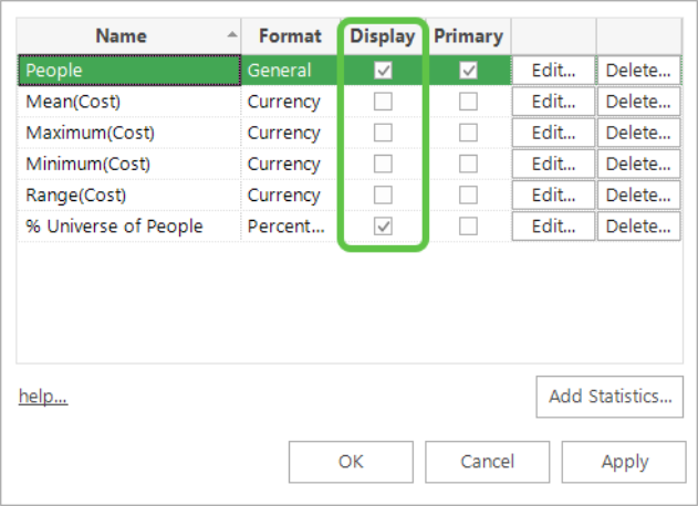
You can show or hide the various options in the list by setting or clearing the Display tickbox.
-
You can also change which quantity the cube is coloured by in the first dialog box. Set the Primary Statistic option for the piece of information you want the thematic shading to be based upon.
-
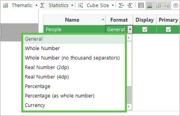
You can also change the way the information is displayed using the display Format drop-down list.
-
Click the Build button to produce the table.
Aggregation functions in a cube
If you have dragged on a variable or expression in step 4, then you will have to choose which function to use to aggregate the values for each record up into each cell of the cube (which will represent multiple records). The options are:
-
Sum to add up all values for all records in this cell.
-
Mean to get the average value for all records in this cell.
-
Populated to get the count of all values in this cell that are not "missing" values..
-
Minimum to get the smallest value for all records in this cell.
-
Maximum to get the largest value for all records in this cell.
-
Median to get the "middle" value for all records in this cell.
-
Variance to measure how far a set of numbers is spread out.
-
Standard Deviation Deviation to get the square root of the variance.
-
Lower Quartile to get the middle number between the smallest number and the median of the data set.
-
Upper Quartile to get the middle value between the median and the highest value of the data set.
-
Inter Quartile Range to get the difference between the upper quartile and the lower quartile.
-
Range to get the difference between the maximum and minimum values of the variable.
-
Mode to get the most frequently occurring value in the data set.
Note that cube statistics can show the Mode average of selector variables as well as numeric variables. The index of the value is returned in the cube because the result of a cube statistic must be numeric. Click here for a worked example.
- Percentile to view values at different points in ordered data.
-
CountDistinct returns a value in this cell for the number of distinct instances of the variable found for the records in that cell - Click here for a worked example.
- Count Mode returns a value in this cell for the number of times the modal value has been found - Click here for a worked example.
- Nth Biggest to return a particular Nth value from the top of the list after all the values in a cell are sorted and ordered.
- Nth Smallest to return a particular Nth value from the bottom of the list after all the values in a cell are sorted and ordered.
Statistics in a cube
The choice of statistics you can display as mentioned in step 5. are as follows. For examples of how to use these statistics, see Cubes: How do I use and interpret the different statistics?
-
Value for the simple value of what has been already specified in the dialog box.
-
% Column calculates the percentage of the value in this cell with reference to the column total.
-
% Row calculates the percentage of the value in this cell with reference to the row total.
-
% Total calculates the percentage of the value in this cell with reference to the total within the red box area – e.g. the percentage of everybody within this 2D sub-cube which forms part of a 3D cube. (See note below)
-
% Grand Total calculates the percentage of the value in this cell with reference to the grand total of the cube – e.g. If resolved to People then the percentage of everybody in this cube.
-
% Universe calculates the percentage of the value in this cell with reference to the number of records in the table the cube resolves to – e.g. If resolved to People, then this is the percentage of everybody in the database.
-
Index calculates an index of the cell value relative to its expected value. See below for a more detailed explanation.
-
Σ Row is the cumulative total along the row, starting from the left hand side.
-
Σ Column is the cumulative total down the column, starting from the left hand side.
-
Σ% Row calculates the percentage of the cumulative total along the row with reference to the total for the row.
-
Σ% Column calculates the percentage of the cumulative total down the column with reference to the total for the column.
-
PWE Predictive Weight of Evidence. This is Apteco's patent pending modelling technique applied to cube results. For more information see the Profiling section.
-
Chi Square measure showing the dependence between two variables. See below for a more detailed explanation.
-
Exp Expected value calculated from row and column totals as a proportion of the grand total. See below for a more detailed explanation.
-
Zd Exp is the standardised measure of how confident we can be that the result presented is a true characteristic of the data and not a quirk of the data sample used. See below for a more detailed explanation.
-
%d Exp Percentage difference from expected value. See below for a more detailed explanation.
Note: All of the above statistics are calculated with reference to the "red box" that they are within. With a 2 dimensional cube (with one row and one column dimension) the whole cube is contained within one red box. However, cubes with more dimensions can be thought of as lots of smaller 2 dimensional cubes appended next to each other. Each of these 2D cubes is highlighted with a red box.
For example, consider the three dimensional cube of Gender v Income v Occupation.
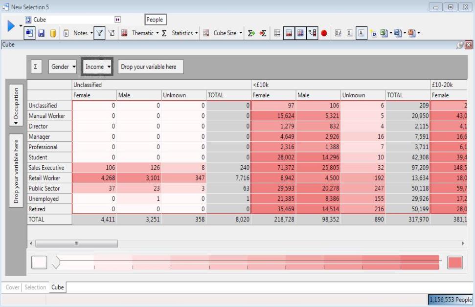
This 3D cube is effectively a 2D cube of Gender v Occupation for Income of "Unclassifed", placed alongside another 2D cube of Gender v Occupation for Income of "<10k", and another of Gender v Occupation for Income of "10k - 20k", and so on. You can see that the part of the cube that shows Gender v Occupation for Income of "Unclassified" is surrounded by a red box.
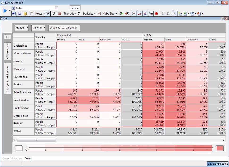
When statistics are added to the cube (such as % Row, below) they are calculated within the red box that makes up the innermost 2D cube. For example, the % Row value for male public sector workers with an unknown income is 36.51%, which is the number of male public sector workers with an unclassified income (23), as a percentage of all public sector workers with an unknown income (63). This shows that the statistics shown don't take account of values outside of their red box, such as numbers of people with known incomes, such as less than 10K, etc.
To explain how the more advanced statistics on a cube work, consider the following table:
|
|
Column 1 |
Column 2 |
... |
Column m |
Column Total
|
|
Row 1 |
Cell11 |
Cell12 |
... |
Cell1m |
Cell1+ |
|
Row 2 |
Cell21 |
Cell22 |
... |
Cell2m |
Cell2+ |
|
... |
... |
... |
... |
... |
... |
|
Row n |
Celln1 |
Celln2 |
... |
Cellnm |
Celln+ |
|
Row Total |
Cell+1 |
Cell+2 |
... |
Cell+m |
Cell++ |
This shows a table with n rows and m columns. The data cells are shown in the table as Cellnm to indicate the value in the nth row and mth column. The last row and last columns then show subtotals for the table. For example, Cell+2 is the subtotal for the 2nd column (i.e. the sum of all the values for Cell12, Cell22, ..., Celln2). Cell++ is the grand total, totaling up all cell values for the table.
The functions described above are as follows:
-
Exp(Cellxy) = ( Cell+y * Cellx+ ) / Cell++
-
Index(Cellxy) = ( Cellxy / Exp(Cellxy) ) * 100
-
ChiSquare(Cellxy) = ( Cellxy - Exp(Cellxy) )2 / Exp(Cellxy)
-
%dExp(Cellxy) = ( ( Cellxy - Exp(Cellxy) ) / Exp(Cellxy) ) * 100
-
ZdExp(Cellxy) = Z(Cellxy) / V(Cellxy)0.5
Where:
- Z(Cellxy) = ( Cellxy - Exp(Cellxy) ) / Exp(Cellxy)0.5
- V(Cellxy) = ( 1 - ( Cell+y / Cell++) ) * ( 1 - ( Cellx+ / Cell++) )